OLC

OLC算法由张承玺博士提出，本文主要参考其首次提出OLC算法的论文On low-complexity control design to spacecraft attitude stabilization: An online-learning approach。OLC和NON-OLC的控制律参考该论文，控制对象选取一般二阶对象。

Compared with the conventional control design, an obvious distinction of the online-learning control (OLC) algorithm is that it together utilizes the previous control input information and the system’s current state information, as if learning experience from previous control input. In contrast, the conventional control scheme does not fully use the existing information and chooses to discard the previous control input information when generating control instructions. Due to the learning strategy, the utility of adaptive- or observer-based tools can be avoided when designing a robust control law, making a simple, effective algorithm, moreover saving system resources.

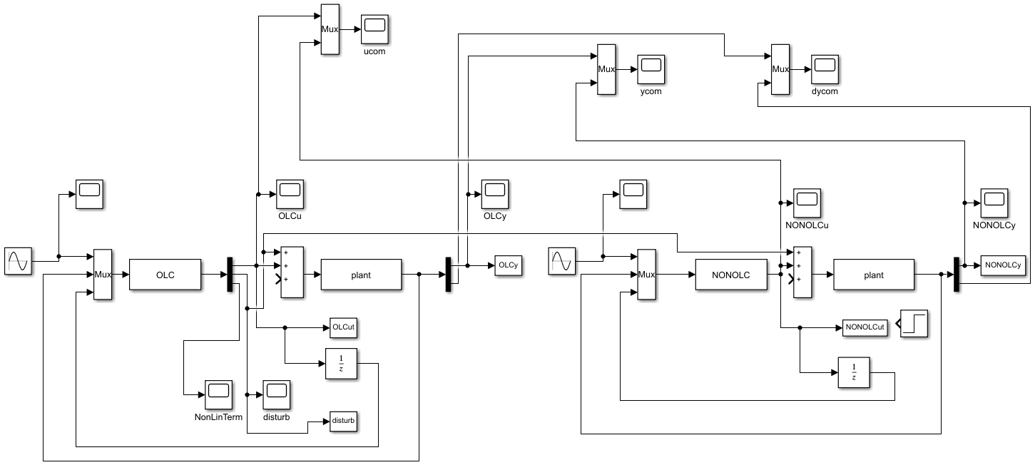
OLC是一种简单易用的控制算法，具有一定的工程实践意义。本例程采用MATLAB Simulink进行仿真，包含三个S-Function：二阶控制对象、OLC控制器、NON-OLC控制器。

控制对象

随便选了一个二阶对象，代码如下：

function [sys,x0,str,ts]=plant(t,x,u,flag)
switch flag,
case 0,
    [sys,x0,str,ts]=mdlInitializeSizes;
case 1,
    sys=mdlDerivatives(t,x,u);
case 3,
    sys=mdlOutputs(t,x,u);
case {2, 4, 9 }
    sys = [];
otherwise
    error(['Unhandled flag = ',num2str(flag)]);
end
function [sys,x0,str,ts]=mdlInitializeSizes
sizes = simsizes;
sizes.NumContStates  = 2;
sizes.NumDiscStates  = 0;
sizes.NumOutputs     = 2;
sizes.NumInputs      = 1;
sizes.DirFeedthrough = 0;
sizes.NumSampleTimes = 0;
sys=simsizes(sizes);
x0=[0.5 0];
str=[];
ts=[];

function sys=mdlDerivatives(t,x,u)
I=0.4958;
Dyal=(2.2265-1.3735)*rand(1)+1.3735;
Delta=(0.4265-(-0.4265))*rand(1)+(-0.4265);
D=Dyal+Delta;
sys(1)=x(2);            %dx
sys(2)=1/I*(u-D*x(2));  %ddx

function sys=mdlOutputs(t,x,u)
sys(1)=x(1);
sys(2)=x(2);

OLC控制器

将外部干扰的轨迹写在这个S-Function里面，形如：

外部干扰信号

同时也包含OLC控制器本身，代码如下：

function [sys,x0,str,ts] = OLCctrl(t,x,u,flag)

switch flag,
case 0,
    [sys,x0,str,ts]=mdlInitializeSizes;
case 3,
    sys=mdlOutputs(t,x,u);
case {2,4,9}
    sys=[];
otherwise
    error(['Unhandled flag = ',num2str(flag)]);
end

function [sys,x0,str,ts]=mdlInitializeSizes
sizes = simsizes;
sizes.NumOutputs     = 3;
sizes.NumInputs      = 4;
sizes.DirFeedthrough = 1;
sizes.NumSampleTimes = 1;
sys = simsizes(sizes);
x0  = [];
str = [];
ts  = [0 0];

function sys=mdlOutputs(t,x,u)

xd=0;           %xd期望值
dxd=0;     
ddxd=0;
xr=u(2);        %xr实际值
dxr=u(3);

e=xr-xd;        % x tilt
de=dxr-dxd;     % x tilt的微分

I=0.4958;
Dn=2.2625;      %D的名义值
Delta=(0.4265-(-0.4265))*rand(1)+(-0.4265);
DB=abs(Delta);
Eta=15;         %参数η的取值
k=DB*abs(dxr)+I*Eta;
lamd=10;        %参数λ的取值
s=de+lamd*e;	%定义滑模面

% 控制输入u
uttau= - k*s;
NonLinTerm=Dn*dxr + I*ddxd - I*lamd*(dxr-dxd);

ut=0.8*u(4)+2*uttau;

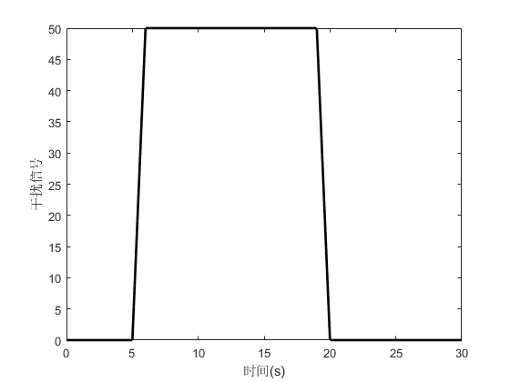
% 干扰为梯形脉冲信号
if (t<5)
    disturb=0;
elseif (t>=5 & t<=6)
    disturb=50*t-250;
elseif (t>6 & t<19)
    disturb=50;
elseif (t>=19 & t<=20)
    disturb=-50*t+1000;
else
    disturb=0;
end

sys(1)=ut;
sys(2)=disturb;
sys(3)=NonLinTerm;

NON-OLC控制器

NON-OLC控制器的控制律形式与OLC的类似，只不过是去掉了学习项。相比于上一个S-Funcion，也去掉了干扰信号。代码如下：

function [sys,x0,str,ts] = NONOLCctrl(t,x,u,flag)

switch flag,
case 0,
    [sys,x0,str,ts]=mdlInitializeSizes;
case 3,
    sys=mdlOutputs(t,x,u);
case {2,4,9}
    sys=[];
otherwise
    error(['Unhandled flag = ',num2str(flag)]);
end

function [sys,x0,str,ts]=mdlInitializeSizes
sizes = simsizes;
sizes.NumOutputs     = 1;
sizes.NumInputs      = 4;
sizes.DirFeedthrough = 1;
sizes.NumSampleTimes = 1;
sys = simsizes(sizes);
x0  = [];
str = [];
ts  = [0 0];

function sys=mdlOutputs(t,x,u)

xd=0;           %xd期望值
dxd=0;     
ddxd=0;
xr=u(2);        %xr实际值
dxr=u(3);

e=xr-xd;        % x tilt
de=dxr-dxd;     % x tilt的微分

I=0.4958;
Dn=2.2625;      %D的名义值
Delta=(0.4265-(-0.4265))*rand(1)+(-0.4265);
DB=abs(Delta);
Eta=15;         %参数η的取值
k=DB*abs(dxr)+I*Eta;
lamd=10;        %参数λ的取值
s=de+lamd*e;	%定义滑模面

uttau= - k*s;
ut=2*uttau;

sys(1)=ut;

SIMULINK仿真

仿真图包含OLC和NON-OLC两部分，只是示波器连在了一起，并且通过To Workspace将仿真后的结果导出。

Simulink仿真图

正弦波作为输入信号可以用于设定跟踪轨迹，而本次仿真将OLC作为简单的镇定器来使用，因此设定值及其导数为0。

结果

将Workspace里面的数据画成图片，代码如下：

close all;

figure(1);
plot(t,disturb,'k','linewidth',2);
xlabel('时间(s)');ylabel('干扰信号');

figure(2);
plot(t,NONOLCut,'linewidth',2,'Color',[0.5 0.5 0.5]);
hold on;
plot(t,OLCut,'r','linewidth',1);
xlabel('时间(s)');ylabel('控制输入信号');
legend('NON-OLC','OLC');

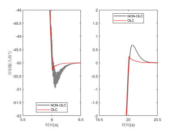
figure(3);
subplot(1,2,1); 
plot(t,NONOLCut,'linewidth',2,'Color',[0.5 0.5 0.5]);
hold on;
plot(t,OLCut,'r','linewidth',1);
axis([5.5 6.5 -52 -48])
xlabel('时间(s)');ylabel('控制输入信号');
legend('NON-OLC','OLC','location','South');

subplot(1,2,2); 
plot(t,NONOLCut,'linewidth',2,'Color',[0.5 0.5 0.5]);
hold on;
plot(t,OLCut,'r','linewidth',1);
axis([19.5 20.5 -2 2])
xlabel('时间(s)');%ylabel('控制输入信号');
legend('NON-OLC','OLC','location','North');

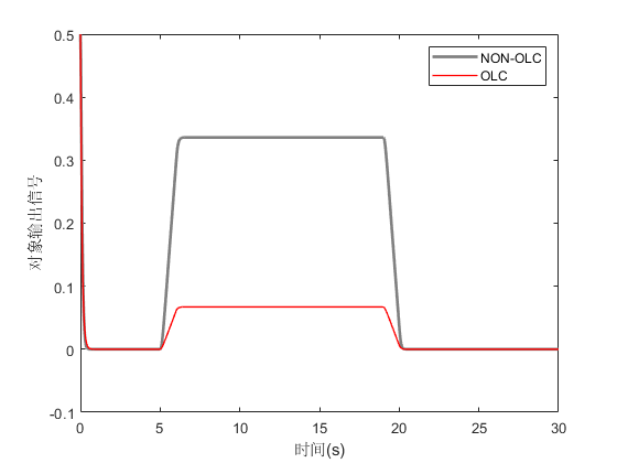
figure(4);
plot(t,NONOLCy,'linewidth',2,'Color',[0.5 0.5 0.5]);
hold on;
plot(t,OLCy,'r','linewidth',1);
xlabel('时间(s)');ylabel('对象输出信号');
legend('NON-OLC','OLC');

对象输出

可以看出，面对幅值为50的干扰信号，NON-OLC仅能将输出信号y压到0.4以内，但是OLC可以压到0.1以下。

对象输出信号的结果对比图

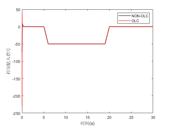
控制输入

OLC在0时刻的控制输入u变化较为剧烈，在多数情况下，考虑到实际执行器的非线性、时滞等因素，该行为并不会对被控对象产生实质性影响，这一点从上述输出信号y的对比中也能看出。总体来看，OLC的控制输入u与NON-OLC基本重合，如下图所示：

控制输入信号对比图

放大看细节不难发现，OLC的优势相比于NON-OLC还是很明显的，不管是从超调情况，还是噪声摆幅方面。

控制输入信号放大对比

Online learning control for stabilization

A novel and efficient control algorithm

OLC